 (11.1)
The development of digital synthesis and processing owes a great deal to the ‘classic’ techniques employed in the early years of electroacoustic music. These involved processes which, in most cases, were based on the capabilities of analog devices. Even today, when the flexibility offered by digital systems allows tighter control of spectral characteristics and application of sophisticated mathematical models, the theoretical principles underpinning the ‘classic’ processes still offer a powerful set of tools for the achievement of complex morphologies, which is greatly enhanced by the versatility of the new technology.
‘Classic’ techniques may be categorized according to the principles involved in their realization, as shown in the figure 11.1.
|
Additive synthesis
|
|||
|
Linear
|
|||
|
Subtractive synthesis
|
|||
|
Frequency-domain
|
Ring modulation
|
||
|
Amplitude modulation
|
|||
|
Non-linear
|
Waveshaping
|
||
|
Frequency modulation
|
|||
|
Time-domain
|
(Non-linear)
|
Granular synthesis
|
|
Figure 11.1 Classic synthesis techniques classified according to their principles of realization.
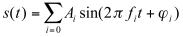
Frequency-domain techniques are based on the assumption that any signal can be considered to be the sum of sines or cosines — each with its own amplitude, frequency and phase — according to theoretical principles developed by Fourier (1768-1830). Mathematically, this may be expressed as follows:
(11.1)
where Ai, fi and j i are, respectively, the amplitude, frequency and phase of the ith sinewave.
On the other hand, granular synthesis is a time-domain technique based on the construction of signals from the combination of very short sounds, called grains.
Linear techniques are processes that do not distort the input and, as a consequence, do not create new frequencies that were not already contained in the input before it was processed. Linear procedures process signals in three possible ways: delay of samples, scaling (which is equivalent to multiplying a sample by a constant) and addition or subtraction of scaled samples (which may or may not have been delayed).
Non-linear techniques consist of the controlled distortion of a signal, which results in the creation of frequencies not found before the latter was processed. This can be achieved in various ways. For example, it is possible to use a signal in order to modify the amplitude of another (amplitude modulation) by multiplying the former by the latter. Alternatively, a signal may be used to modify the frequency of another (frequency modulation).
We will now proceed to examine the various techniques in more detail.
Additive Synthesis
Additive processes consist of synthesis by means of a direct implementation of equation 11.1 above. Sinewaves of various frequencies and amplitudes are added together (mixed) in order to produce complex sounds. This is illustrated in
.orc and 1101.sco. The former consists of the following instrument:
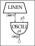
Figure 11.2 Block diagram of instr 1101, a simple oscillator instrument with an amplitude envelope.
            instr         1101                   ; simple oscillator
kenv        linen         p4, 0.1, p3, 0.2       ; envelope
asig        oscili        kenv, p5, p6           ; oscillator
            out           asig                   ; output
            endin
Figure 11.3 Orchestra code for instr 1101, a simple oscillator instrument
Instr 1101 contains a simple oscillator that may produce a single sinewave or a combination of components, depending on the type of waveform defined by the f-table (p6). The maximum amplitude, determined by p4, is fed to an envelope generator (kenv), which controls the amplitude of the oscillator. The frequency of the oscillator is given by p5. The attack is 0.1 beats and the decay is 0.2 beats.
The score produces the following sounds. First, the individual components of a bassoon-like sound, based on data presented by Backus (1977, p 116), are played separately. These are then superimposed in ascending frequency order. At this point it is possible to appreciate how the overall timbre changes as components are added. Finally, they are all mixed together in order to produce the synthetic ‘bassoon’, which is used in a short musical passage from The Sorcerer’s Apprentice, by Dukas.
The individual components are generated by f 1 using GEN10:
| f 1 | 0 | 8192 | 10 | 1 |
The waveform in the ‘bassoon’ passage of the final section of this example is generated with f 2, which uses GEN10 to produce a waveform resulting from combining eight components, each with its own relative amplitude:
| f 2 | 0 | 8192 | 10 | .24 .64 .88 .76 .06 .5 .24 .08 |
In its simplest form, additive synthesis may be used to produce a static spectrum. This is a combination of sines and cosines in which the amplitude and frequency of each component remain unchanged throughout the duration of the sound. Within these constraints, timbral identity is determined by the particular set of relative amplitudes, frequencies and — to a lesser extent — phases of the components. For example, consider the following sounds:
| Sound 1 | Sound 2 | Sound 3 | ||||||||
| Amp. | Freq.(Hz) | Amp. | Freq.(Hz) | Amp. | Freq.(Hz) | |||||
| 500 | 100 | 1000 | 110 | 3500 | 110 | |||||
| 750 | 200 | 1500 | 220 | 3000 | 330 | |||||
| 1000 | 300 | 2000 | 330 | 2500 | 550 | |||||
| 1250 | 400 | 2500 | 440 | 2000 | 770 | |||||
| 1000 | 500 | 2000 | 550 | 1500 | 990 | |||||
| 750 | 600 | 1500 | 660 | 1000 | 1210 | |||||
| 500 | 700 | 1000 | 770 | 500 | 1430 | |||||
Figure 11.4 The static spectra of three additive synthesis sounds.
Close inspection of sounds 1 and 2 reveals that their frequency components have relative ratios 1, 2, 3, 4, 5, 6 and 7, namely:
| 200 | = | 2 x 100 | and | 220 | = | 2 x 110 |
| 300 | = | 3 x 100 | 330 | = | 3 x 110 | |
| 400 | = | 4 x 100 | 440 | = | 4 x 110 | |
| etc. | etc. |
The same happens to the corresponding amplitudes, which have relative ratios 1, 1.5, 2, 2.5, 2, 1.5, and 1. Therefore, we expect these sounds to have the same timbre (and different pitch), in spite of the fact that they do not have any common frequency components. On the other hand, the frequency ratios in sound 3 are 1, 3, 5, 7, 9, 11, 13 and the relative amplitudes are 7, 6, 5, 4, 3, 2, 1. These are not the same as sound 2; thus in spite of having some common frequencies with the latter, sound 3 has a different timbre. Sounds 1, 2 and 3 are realized in 1102.orc and 1102.sco. The orchestra uses instr 1102, which is similar to instr 1101, except for the fact that p6 and p7 indicate the attack and decay and p8 indicates the function table.
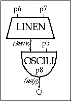
Figure 11.5 Block diagram of instr 1102, a variable waveform oscillator instrument.
| instr | 1102 | ; simple oscil with amp env | ||
| kenv | linen | p4, p6, p3, p7 | ; envelope | |
| asig | oscili | kenv, p5, p8 | ; oscillator | |
| out | asig | ; output | ||
| endin | ||||
Figure 11.6 Orchestra code for instr 1102, a variable waveform single oscillator instrument with variable attack and release amplitude envelopes
The score file 1102.sco implements the spectrum of sounds 1, 2 and 3 above using the following function tables:
| f 1 | 0 | 8192 | 10 | 500 750 1000 1250 1000 750 500 |
| f 2 | 0 | 8192 | 10 | 1000 1500 2000 2500 2000 1500 1000 |
| f 3 | 0 | 8192 | 10 | 3500 0 3000 0 2500 0 2000 0 1500 0 1000 0 500 |
Figure 11.7 Harmonically complex f-tables for use in instr 1102.
Frequency ratios may also determine whether a signal has pitch. If f is the lowest frequency component of a sound its spectrum is said to be harmonic when all other components are integer multiples of f. In this case, the sound will normally have definite pitch determined by f, which is called the fundamental. The components are then said to be harmonics: the first harmonic is f, the fundamental; the second harmonic is 2f, the third 3f and so on. When the relative frequencies of the components are not integer multiples of f, the spectrum is inharmonic and it is more difficult to recognize pitch. Increasing deviation from harmonic ratios causes sounds to become less pitched. The files 1103.orc and 1103.sco demonstrate this: the first event is a sound with a 280 Hz fundamental and six additional harmonics with relative amplitudes 1, 0.68, 0.79, 0.67, 0.59, 0.82 and 0.34. This is followed by an inharmonic sound in which the lowest component is also f = 280 Hz but the other six are not integer multiples of f but rather 1.35f, 1.78f, 2.13f, 2.55f, 3.23f and 3.47f. In spite of the fact that the relative amplitudes of the components are kept, the second sound does not resemble the first and has no definite pitch due to the fact that its spectrum is inharmonic.
In order to implement a sound with seven components, instr 1103 uses seven oscillators that are subsequently mixed and multiplied by the overall envelope (kenv).

Figure 11.8 Block diagram of instr 1103, a seven partial additive synthesis instrument with common amplitude envelope.
The relative amplitudes of the components are given in p6, p8, p10, p12, p14, p16 and p18. The frequencies of the oscillators are obtained multiplying the reference frequency f (given by p5) by the component ratios specified in p7, p9, p11, p13, p15, p17 and p19. For example, if f = 280 Hz and the second component has a relative amplitude of 1 and a frequency ratio of 1.35, the values of p5, p8 and p9 will be 280, 1 and 1.35, respectively. The oscillator producing this component will be:
| a1 | oscil | p8, p5*p9, 1 | ; 1st component |
And the components are mixed using the following statement:
| out | kenv*(a1+a2+a3+a4+a5+a6+a7)/7 | ; mix and output |
So far, the discussion has focused on static spectrum. However, most sounds in nature have dynamic spectra, whereby the amplitude and frequency of each component change throughout duration of a sound. This means that Ai, fi and j i in equation 11.1 are time-dependent.
Using additive synthesis in order to achieve dynamic spectrum may become a laborious task given the amount of data involved. Convincing results may sometimes require the use of a large number of components, each of which requires independent amplitude, frequency and phase control. In 1104.orc and 1104.sco I present an example of dynamic spectrum synthesis realized with an instrument which employs six oscillators, each with variable amplitude and frequency. In addition, the output is spatialized. The amplitude and frequency of each component vary by a percentage specified respectively in p8 and p9. These are translated into fractions using the following statements:
| imaxaf | = | p8/100.00 | ; maximum amplitude fluctuation |
| imaxff | = | p9/100.00 | ; maximum frequency fluctuation |

Figure 11.9 Block diagram of a six component additive synthesis instrument with variable amplitude and frequency of each partial, plus a group envelope and panning
The implementation of each component takes account of these fluctuations by including time-varying controllers for amplitude and frequency. For example, the first component is implemented using the following set of statements:
| iramp1 | = | p10 | ; relative amplitude | |
| imaxaf1 | = | iramp1*imaxaf | ; maximum amp fluctuation | |
| iafunc1 | = | p12 | ; amplitude fluctuation fn | |
| ifreq1 | = | p11*ifreq | ; frequency | |
| imaxff1 | = | ifreq1*imaxff | ; maximum freq fluctuation | |
| iffunc1 | = | p13 | ; frequency fluctuation fn | |
| kampf1 | oscil1 | 0,imaxaf1,idur,iafunc1 | ; Amplitude Control | |
| kfreqf1 | oscil1 | 0,imaxff1,idur,iffunc1 | ; Frequency Control | |
| a1 | oscil1 | iramp1+kampf1, ifreq1+kfreqf1, 1 | ; oscillator | |
Figure 11.10 Orchestra code for the first component of additive instrument shown in figure 11.9.
Amplitude fluctuation is controlled by kampf1 according to a function table given by iafunc1. The maximum value of kampf1 is imaxaf1, which is calculated as a fraction of iramp1, the relative amplitude of the component specified in the score. Therefore, adding kampf1 to iramp1 in the oscili statement means that the actual relative amplitude will fluctuate around iramp1 depending on the shape of iafunc1. A similar procedure uses kfreqf1 and ifreqf1 to control the frequency of the component.
Components are mixed using the following statements:
| iampsum | = | iramp1+iramp2+iramp3+iramp4+iramp5+iramp6 | ; max amplitude |
| asig | = | kenv*(a1+a2+a3+a4+a5+a6)/(iampsum) | ; balanced mix |
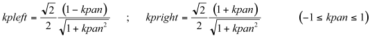
In order to spatialize the output, the number of channels is set to 2 in the header (nchnls= 2), an outs statement is used instead of out and asig is multiplied by time-varying scaling factors kpleft and kpright before it is sent to the left and right channels:
| outs | kpleft*asig, kpright*asig | ; OUTPUT |
kpleft and kpright are calculated according to the following algorithm: if kpan is the instantaneous position along the line joining the speakers, kpan = -1 and kpan = 1 represent respectively the positions of the left and right speakers. Values between -1 and 1 represent positions between the speakers (kpan = 0 is the center). Values below -1 represent positions beyond the left speaker.
If the source is between the speakers then:
 (11.2)
If the source is beyond the left speaker:
 (11.3)
If the source is beyond the right speaker:
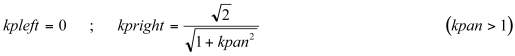 (11.4)
The statement generates the spatial trajectory of the output:
| kpan | oscil1 | 0, imaxpan, idur, ipanfunc | ; panning trajectory |
where imaxpan is 2 and ipanfunc (p34) is the function table determining the shape of the trajectory. Since there are different formulas for the position of the source, the instrument must check the value of kpan and decide which formula to apply using if ... kgoto statements.
| if kpan < -1 kgoto beyondl | ; chk pan beyond left spkr | ||
| if kpan >1 kgoto beyondr | ; chck pan beyond right spkr | ||
| ktemp | = | sqrt(1+kpan*kpan) | ; pan between speakers |
| kpleft | = | isr2b2*(1-kpan)/ktemp | |
| kpright | = | isr2b2*(1+kpan)/ktemp | |
| kgoto | donepan | ||
| beyondl: | ; pan beyond left speaker | ||
| kpleft | = | 2.0/(1+kpan*kpan) | |
| kpright | = | 0 | |
| kgoto | donepan | ||
| beyondr: | ; pan beyond right speaker | ||
| kpleft | = | 0 | |
| kpright | = | 2.0/(1+kpan*kpan) | |
| donepan: | |||
Figure 11.11 Orchestra code excerpt for panning algorithm supporting both an equal-power pan and a wide-stereo effect.
Summary
Additive synthesis may be used to create dynamic spectra. Each component requires the following parameters:
1. Amplitude envelope.
2. Time-varying frequency.
Subtractive Synthesis
This is the counterpart of additive procedures. While the latter constructs spectra using single sinewaves in order to implement the equation, subtractive synthesis uses complex spectra as inputs which are shaped by enhancing or attenuating the component sinewaves, as illustrated in figure 11.12. Mathematically, this means that the values of Ai in equation 11.1 are modified.
The output depends on the choice of sources and the behavior of the filters. In fact, because of the power loss due to the attenuation of components, some type of amplification may be required after.
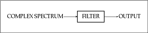
Figure 11.12 Block diagram of a basic subtractive synthesis system.
The main consideration regarding choice of sources is their spectral content. If we intend to process frequencies in a certain region of the spectrum, it is important to ensure that these frequencies exist in the source; otherwise there will be nothing to filter. For this reason, noise and trains of pulses are frequently used, since they offer a uniform spread of components throughout the auditory range.
Ideal white noise is probably the richest available source. For practical purposes, it is possible to consider it as a signal that contains all frequencies evenly distributed throughout the auditory range. White noise is normally obtained using a generator that produces a random number every sample. The aural result is rather like a hiss.
An ideal train or sequence of pulses consists of a signal containing an infinite number of harmonics, all of which have the same relative amplitude. In practice, approximations of a pulse sequence may be obtained by combining as many harmonics as possible up to the upper threshold of the auditory range. It is also important to consider the limitations imposed by the sampling rate sr (according to the sampling theorem, the highest frequency sampled with sr must be less than sr/2). The file 1105.orc consists of instruments that produce white noise and trains of pulses. For instr 1105 a rand generator is used to produce white noise as shown in figure 11.13.
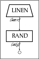
Figure 11.13 Block diagram of instr 1105, a white noise generator.
| instr | 1105 | ; env controlled white noise | ||
| kenv | linen | p4, p6, p3, p7 | ; envelope | |
| asig | rand | kenv | ; noise source | |
| out | asig | ; output | ||
| endin | ||||
Figure 11.14 Orchestra code for instr 1105, an envelope controlled white noise instrument.
For instr 1106 a buzz is used to produce a train of pulses with as many harmonics as possible given the sampling rate (sr). If the frequency of the fundamental is p5, then the frequency of the nth harmonic is n times p5. This frequency must be less than sr/2; therefore, the maximum number of harmonics, iinh, must be equal or less than sr/2/p5. Since the number of harmonics must be an integer, the operator int is used in order to calculate iinh. Figure 11.15 shows a block diagram of instr 1106.
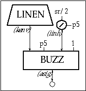
Figure 11.15 Block diagram of instr 1106, a buzz (pulse train) instrument with an amplitude envelope.
| instr | 1106 | ; pulse train w/ amp env. | ||
| iinh | = | int(sr/2/p5) | ; maximum number of harmonics | |
| kenv | linen | p4, p6, p3, p7 | ; envelope | |
| asig | buzz | kenv, p5, iinh, 1 | ; oscillator | |
| out | asig | ; output | ||
| endin | ||||
Figure 11.16 Orchestra code for instr 1106, a buzz instrument with controls for the number of harmonics in the pulse-train.
The file 1105.sco produces white noise (instr 1105) followed by a train-of-pulses (a pulse-train instr 1106) with a fundamental of 75 Hz.
Filters are characterized by their response, which represents the frequency regions they attenuate and enhance. Figure 11.17 shows the four ideal types of filters used in subtractive synthesis. These are classified as follows:
1. Filters that only pass frequencies above a cut-off value fc, or highpass.
2. Filters which only pass frequencies below fc, or lowpass.
3. Filters which only pass components with frequencies inside a band above and below a center frequency fc, or bandpass. The size in Hz of the bandpass is the bandwidth (bw).
4. Filters which only pass components with frequencies outside a band above and below a center frequency fc, or bandreject.
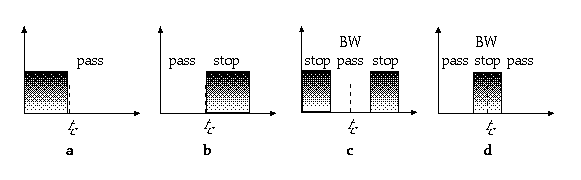
Figure 11.17 Ideal filter types. (a) Highpass. (b) Lowpass. (c) Bandpass. (d) Bandreject.
The four filter types shown in figure 11.17 represent ideal filters. In practice, the transition between pass and stop regions is not as sharp as in figure. Its slope is known as the roll-off and is measured in decibels per octave, which is the change in attenuation when the frequency is doubled. The fact that there is a slope means that the cut-off frequency must be re-defined as the value at which the attenuation is -3 dB, which is equivalent to a drop in amplitude by a factor of about 0.71.
In order to achieve sharper responses, filters may be cascaded by using the output of one filter as the input of another. Filters may also be connected in parallel, with two or more filters sharing the same input and having their outputs mixed into one signal; thus achieving complex response curves. Cascade and parallel connections are shown in figure 11.18.

Figure 11.18 Filter connections. (a) Cascade. (b) Parallel.
We have seen above that in order to achieve a dynamic spectrum it is necessary to vary the amplitudes and frequencies of components in time. Linear filters cannot alter the frequencies of the components of a source; however, they can change their amplitudes. This may be done by varying the cut-off frequency in low and highpass filters and by varying the center frequency and bandwidth in bandpass and bandreject filters.
As an example, the files 1107.orc and 1107.sco produce sounds resembling vowel articulation by modeling the mechanism driving the vocal chords: a rich pulse (maximum possible harmonics) is passed through five parallel bandpass filters.
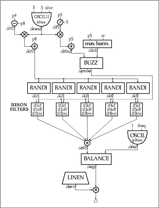
Figure 11.19 Block diagram of instr 1107, a parallel, pseudo-random, formant-filter instrument.
Their center frequency and bandwidth fluctuate randomly in the vicinity of values corresponding to the filtering processes in human speech. The rate at which the random numbers are generated is varied between a minimum (irfmin) and a maximum (p9), according to the control variable krfl:
| irfmin | = | p8 | ; minimum random rate |
| itfl | = | p9-p8 | ; maximum fluctuation |
| irfunc | = | 2 | ; fluctuation function |
| ... | |||
| ... | |||
| krand | oscil1i | 0, .5, idur, irfunc | ; oscil between -.5 and .5 |
| krand | = | krand+.5 | ; correct between 0 and 1 |
| krfl | = | irfmin+irfl*krand | ; RATE of RANDOM GENERATORS |
Each filter uses a randi generator in order to produce center frequency and bandwidth fluctuations. For example, the first formant is controlled by k1, which is multiplied by the maximum center frequency fluctuation, if1cff and added to a minimum center frequency if1cf. The bandwidth is controlled similarly:
| k1 | randi | 1, krfl, .12 | ; random generator |
| ... | |||
| ... | ; first formant | ||
| afilt1 | reson | apulse, if1cf+k1*if1cff, if1bw*(1+k1), 0 | |
The input to the formant filter is apulse, a train of pulses generated using buzz. Its fundamental frequency is made to fluctuate by up to 1/5 of its value. This process is controlled by krand, which is scaled by iffl — the maximum frequency fluctuation and added to ifreq — the minimum frequency value, to produce kfrnd, the frequency input to the pulse generator:
| ifreq | = | p5 | ; frequency of fundamental |
| iffl | = | p5/5 | ; maximum frequency fluctuation |
| iinh | = | int(sr/2/(p5+iffl)) | ; maximum number of harmonics |
| iplfunc | = | 1 | ; function table for BUZZ (sine) |
| ... | |||
| ... | |||
| kfrnd | = | ifreq+iffl*krand | ; frequency fluctuation |
| apulse | buzz | 1, kfrnd, iinh, iplfunc | ; pulse generator |
Figure 11.20 Orchestra code excerpt from instr 1107, a pulse-train generator with fluctuating frequency.
Finally, the filtered pulses are mixed, balanced with a sinewave and sent to the output:
| afilt | = | afilt1+afilt2+afilt3+afilt4+afilt5 | ; mix filtr out |
| abal | oscil | 1, ifreq, iplfunc | ; sinewave control sig |
| asig | balance | afilt, abal | ; output balance |
| out | kenv*asig | ||
Summary
There are three important factors that must be considered in order to obtain dynamic spectra using subtractive procedures:
1. Choice of source (may be time varying). White noise or a pulse-train are commonly used.
2. Time varying filters.
3. Output balance.
Ring Modulation
This non-linear technique consists of the use of a signal, the modulator, used to modify the amplitude of another signal, the carrier. Each sample of the modulator multiplies a corresponding sample of the carrier, distorting the latter and creating new spectral components.
The simplest case of amplitude modulation is that of a sinewave which multiplies another sinewave. If the frequencies of the carrier and modulator are, respectively, fm and fc, the output is:
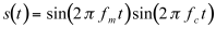 (11.5)
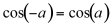
But, from the trigonometric identity for the product of two sines, we have:
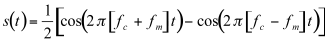 (11.6)
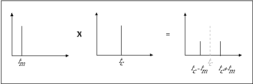
The equation above represents a spectrum containing two components with frequencies fc+fm and fc-fm. These are called sidebands, because they appear on both sides of the carrier, as shown in figure 11.21.
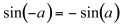
The modulation process requires caution. In the first place, it is important to ensure that fc+fm does not exceed half of the sampling rate (sr/2) in order to comply with the sampling theorem, avoiding aliasing, which causes frequencies over sr/2 to reflect, appearing to be lower, thus assuming a different spectral ‘identity.’ Secondly, if fc and fm are very close, their difference may be below the auditory range; this occurs when fc-fm is below about 20 Hz. If fc is larger than fm, the difference will be a negative number. But from the identity:
 (11.7)
We can infer that only the absolute value of the difference is important and that the sign can be ignored. In other words, a negative frequency reflects as a positive one.
Figure 11.21 Spectrum of simple amplitude modulation
A simple implementation of an amplitude modulator consists of two oscillators, a carrier and a modulator, which have their outputs multiplied:

Figure 11.22 Block diagram of instr 1109, an amplitude modulation instrument with amplitude envelope.
| instr | 1109 | ; simple am | ||
| kenv | linen | p4, p6, p3, p7 | ; envelope | |
| acarr | oscili | 1, p5, p9 | ; carrier | |
| amod | oscili | 1, p8, p9 | ; modulator | |
| asig | = | acarr*amod | ; modulation | |
| out | kenv*asig | ; output | ||
| endin | ||||
Figure 11.23 Orchestra code for instr 1109, the amplitude modulation instrument shown in figure 11.22
The effects of modulation using sinewaves are shown in 1109.orc and 1109.sco. The orchestra consists of two instruments: instr 1108 is identical to instr 1101 and is used to produce separate pairs of sinewaves. Whereas instr 1109 is used to carry out the amplitude modulation by multiplying the sinewaves. The score produces pairs followed by their product, in the following order:
| Sinewave pair | Modulated output | ||||
| Carrier (Hz) | Modulator (Hz) | fc+fm | fc-fm | ||
| 400 | 10 | 410 | 390 | ||
| 400 | 170 | 570 | 230 | ||
| 400 | 385 | 785 | 15 | ||
Figure 11.24 Table of amplitude modulated input signals and output results.
It is worth noticing that the 10 Hz modulator of the first pair is inaudible; however, its effect on the 400 Hz carrier results in two distinct sidebands in the auditory range. Furthermore, the third pair produces a difference sideband of 15 Hz. Therefore, only the 785 Hz component is perceived.
The process above can be extended to signals with several components. For example, the modulator may consist of three frequencies, fm1, fm2 and fm3. Each of these can be considered individually when the modulator is applied to a carrier fc, as illustrated in figure 11.25. Therefore, the output consists of the following pairs:
|
fc + fm1 and fc - fm1
|
fc + fm2 and fc - fm2
|
fc + fm3 and fc - fm3
|

Figure 11.25 Modulator with 3 components
The file 1110.orc consists of instr 1110, a modified version of instr 1109 which allows use of different function tables for both carrier and modulator (the function for the carrier is given in p9 and that for the modulator in p10). The file 1110.sco includes two ring-modulation processes. In the first, a 110 Hz signal with 5 harmonics modulates a 440 Hz carrier. In the second, the same carrier (440 Hz) is modulated with a 134 Hz signal. When synthesized, it is immediately apparent that the first sound is pitched while the second is not. This can be explained by inspection of the output frequencies. The components of the first modulator are 110, 220, 330, 440 and 550 Hz. In the second case, they are 134, 268, 402, 536 and 670 Hz; therefore the components of the respective outputs can be calculated as follows:
| Carrier: 440 Hz - Modulator: 110 Hz | Carrier: 440 Hz - Modulator: 134 Hz | ||||||||
| 440+110 | = 550 | 440-110 | = 330 | 440+134 | = 574 | 440-134 | = 306 | ||
| 440+220 | = 660 | 440-220 | = 220 | 440+268 | = 708 | 440-268 | = 172 | ||
| 440+330 | = 770 | 440-330 | = 110 | 440+402 | = 842 | 440-402 | = 38 | ||
| 440+440 | = 880 | 440-440 | = 0 | 440+536 | = 976 | 440-536 | = -96 | ||
| 440+550 | = 990 | 440-550 | = -110 | 440+670 | = 1110 | 440-670 | = -230 | ||
Figure 11.26 Tables evaluating result of amplitude modulating a complex source, consisting of five harmonics, with a 110 Hz sine wave and a 134 Hz sine wave.
The output of the first sound has the following components; 0 (not heard), 110, 220, 330, 550, 660, 770, 880 and 990 Hz, which produce a harmonic series having a definite pitch. On the other hand, the second output is composed of 38, 96, 172, 230, 306, 574, 708, 842, 976 and 1110 Hz, which produce an inharmonic spectrum.
The example above shows that it is possible to predict harmonicity when the frequencies of carrier and modulator components are known. However, this may be a laborious task when using complex modulators. Obviously, if the modulator is an inharmonic signal, the output will also be inharmonic. If the modulator is harmonic, it is enough to check the result of dividing the carrier by the modulator, called the carrier to modulator ratio, or the c/m ratio. If c/m is an integer, then the carrier is a multiple of the modulator and subtracting or adding the later to fc will create another multiple. Therefore, all the frequencies will be multiples of fm, which will effectively become the fundamental. Similarly, if c/m is of the form 1/n, where n is an integer, the modulator is a multiple of the carrier and, as a consequence, the output frequencies will also be multiples of fc. When c/m deviates from an n/1 or 1/n ratio, the output frequencies become more and more inharmonic. Small deviations (e.g. 1.001) will still produce pitched sounds because the output components will be close to actual harmonic values. In fact, these small deviations produce beating, which may add some liveliness. The effect of the carrier to modulator ratio is shown in 1110a.orc and 1110a.sco. The orchestra consists of instr 10 (described above) and the score contains the following:
1. Hz carrier, 8 harmonic modulator with 300 Hz fundamental (c/m=1).
2. Hz carrier, 8 harmonic modulator with 297.03 Hz fundamental (c/m=1.01).
3. Hz sine carrier, 8 harmonic modulator, 212.13 Hz fundamental (c/m=1.4142~![]() ).
).
Ring modulation can also be used to produce dynamic spectrum. The morphology of the resulting sound can be controlled through the following parameters:
1. Duration.
2. Overall amplitude.
3. Frequency of the carrier.
4. Carrier to modulator ratio, which also determines the modulator frequency from the frequency of the carrier.
5. Fraction of the carrier which is actually modulated (a small percentage will produce less noticeable distortion).
The file 1111.orc contains an instrument that implements time varying: amplitude, carrier-frequency, carrier-to-modulator ratio and modulation-fraction using control variables kamp, kcar, kcmr and kmp.

Figure 11.27 Block diagram of instr 1111, a dynamic Ring-modulation instrument.
| instr | 1111 | ; ring modulation | ||
| ifr | = | cpspch(p5) | ||
| ; ENVELOPES | ||||
| kamp | oscil1 | 0, p4, p3, p7 | ; amplitude | |
| kcar | oscil1 | 0, ifr, p3, p8 | ; carrier freq | |
| kcmr | oscil1 | 0, p6, p3, p9 | ; c/m | |
| kmp | oscil1 | 0, 1, p3, p10 | ; modulation fraction | |
| ; MODULATION | ||||
| acarr | oscili | 1, kcar, 10 | ; carrier | |
| amod | oscili | 1, kcar/kcmr, 11 | ; modulator | |
| aoutm | = | acarr*amod*kmp | ; modulated signal | |
| aoutnm | = | acarr*(1-kmp) | ; unmodulated signal | |
| ; MIX AND OUTPUT | ||||
| out | kamp*(aoutm+aoutnm) | |||
| endin | ||||
Figure 11.28 Orchestra code for instr 1111, a dynamic Ring-modulation instrument with time varying: amplitude, carrier frequency, modulating frequency and modulation ratio.
The functions given by p7, p8, p9 and p10 are fed to control oscillators. The output of the first one, kamp, determines the envelope, with a peak value of p4. The second controls the carrier frequency that can be as high as p5. The third, kcmr, controls the carrier-to-modulator ratio which can reach a maximum of p6. The frequency of the modulator is the product of the carrier-frequency and the carrier-to-modulator ratio.
In order to modulate only part of the carrier, kmp multiplies the modulated carrier acarr*amod, producing aoutm and 1-kmp multiplies the unmodulated carrier, acarr, producing aoutnm. Modulated and unmodulated signals are then mixed and enveloped to produce aout.
The file 1111.sco consists of a short musical excerpt that demonstrates some of the possible sonorities obtainable with instr 1111. It takes advantage of the fact that all the control variables use oscil1, which means that the same function may produce a sharp attack in a very short sound, becoming smeared as the sound becomes longer. This is exactly what happens during the first five beats in the score. Furthermore, the maximum carrier-to-modulator ratio may be altered in the score to produce different timbral shades. This is the case with the fast percussive sounds between beat 5.5 and beat 12.
Summary
The following parameters may be controlled in order to produce diverse sonorities using ring-modulation:
1. Duration.
2. Overall amplitude.
3. Frequency of the carrier.
4. Carrier-to-modulator ratio.
5. Fraction of the carrier which is actually modulated.
Waveshaping
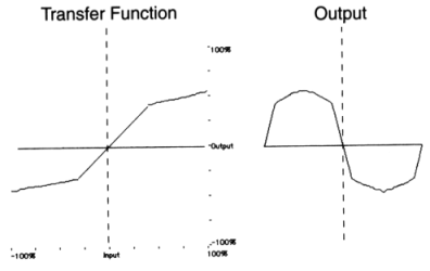
Another way of producing distortion consists of the creation of a dependency between the amplification applied to a sample and its actual value. As you now, at 16 bit, a sample may assume values between 216 = -32,768 and 216-1 = 32,767. So for example, samples with absolute values, under 20,000 may be multiplied by a factor of 1 whereas samples over 20,000 may be multiplied by 0.5; producing compression of the louder parts of a signal, as shown in the following figure:
Figure 11.29 The waveshaping process.
This type of dependency effectively maps the set of possible input values onto a set of output values by means of a transfer function. The general waveshaping process is illustrated in figure 11.30.
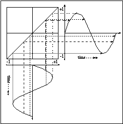
Figure 11.30 Waveshaping of a sinusoidal waveform
Waveshaping may produce various degrees of distortion depending on the chosen transfer function. If the latter approximates a linear device, the effect will not be as pronounced as with more extreme functions. Furthermore, the input may be a fairly simple signal; even sinewaves may be used effectively in order to produce reasonably complex spectra.
A transfer function may be implemented in Csound using the table statement, where the value of a sample is used as the index of the function table as shown in the following block diagram and instrument.
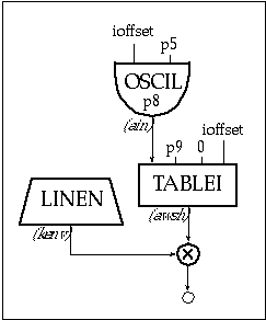
Figure 11.31 Block diagram of instr 1112, a simple waveshaping instrument.
| instr | 1112 | ; simple waveshaping | ||
| ioffset | = | ftlen(p9)/2-1 | ; offset | |
| kenv | linen | p4, p6, p3, p7 | ; envelope | |
| ain | oscil | ioffset, p5, p8 | ; input | |
| awsh | tablei | ain, p9, 0, ioffset | ; waveshaping value | |
| out | kenv*awsh | ; output | ||
| endin | ||||
Figure 11.32 Orchestra code for instr 1112, a simple waveshaping instrument.
The waveshaping table in instr 1112 processes the signal ain. Since the latter can be positive or negative, the upper half of the table processes the positive samples and the lower half the negative ones. Therefore the offset needs to point to the middle of the table. Since the samples are numbered from 0 to the size of the table minus 1, the value of the offset should be half of the table-size minus 1. The table is given by p9 and its size is ftlen(p9).
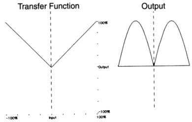
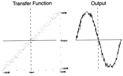
To further clarify the wide range of waveshaping possibilities, figure 11.33 illustrates the waveshaping of a sinewave with a variety of simple and complex transfer functions.
| 
|
| 
|
Figure 11.33 Waveshaping a sinusoid with a variety of simple and complex transfer functions.
The files 1112.orc and 1112.sco make use of instr 1112 in order to demonstrate the difference between near-linear and heavy non-linear processing. Here a sinewave processed by a linear device is heard first (f 2), followed by two waveshaped versions of itself using function f 3 and f 4. The transfer function implementing the linear device is:
| f 2 | 0 | 8192 | 7 | -1 8192 1 |
The transfer functions implementing the non-linear devices are:
| f 3 | 0 | 8192 | 9 | 0.5 1 270 |
| f 4 | 0 | 8192 | 7 | -1 2048 -1 0 0.3 2048 0 -0.5 2048 0 0 0.8 2048 0.8 |
Figure 11.34 Transfer functions for waveshaping.
In general, it is desirable and useful to be able to predict the frequency content of the output in order to control the result of a waveshaping process. It is wise to avoid transfer functions which contain leaps - such as that shown in figure 11.33 above, since these may produce frequencies above half the sampling rate. Instead, smooth functions, which involve relatively simple procedures when evaluating the spectral content of the output, may be used. A family of functions which fits this requirement is the set of polynomials, since, when using a sine for input, the frequency of the highest component produced will be equal to the frequency of the input multiplied by the degree of the polynomial (i.e. the value of its highest power). This may be illustrated by means of an example:
 (11.8)
If the polynomial of the third degree is used as a transfer function that is fed a sinusoidal input of frequency f, we should expect the highest frequency in the output to be 3f. Replacing a sinewave of frequency f, using the trigonometric identity for the sine of three times an angle and performing some algebraic manipulation, we obtain:
 (11.9)
As expected, the highest frequency, 3f, appears in the second term. A further refinement is provided by a family of polynomials that produce a specific harmonic of a sinewave, known as Chebyshev polynomials. The first four Chebyshev polynomials of the first kind are shown below:
T0(x) = 1 the output is a 0 Hz frequency (DC component).
T1(x) = x the output is equal to the input sinewave.
T2(x) = 1-2x2 the output is the second harmonic of the input.
T3(x) = 4x3-3x the output is the third harmonic of the input.
Figure 11.35 The first four Chebyshev polynomials of the first kind.
It is easy to check that these produce the desired harmonics by replacing sin(2¹ft) instead of x in any of the polynomials above. And with the aid of Chebyshev polynomials, it is possible to achieve any combination of harmonics, each with a specified relative amplitude. For instance, if the following combination is required:
| Harmonic | Relative amplitude |
| fundamental | 0.8 |
| 3 | 1 |
| 7 | 0.67 |
| 8 | 0.5 |
Figure 11.36 Table of user specified harmonic number and relative amplitudes.
the transfer function will be:
 (11.10)
So far, the input has consisted of sinusoidals with an amplitude of 1. If the former is multiplied by an amplitude factor K, normalized between 0 and 1, the relative amplitude of the harmonics will be affected. Feeding this type of input to the waveshaper in our equation by using the identity for the sine of 3 times an angle and rearranging terms, will result in the following output:
 (11.11)
Different values of K will produce different relative amplitudes of the fundamental f and the third harmonic 3f. For example, if K = 0.1, the amplitude of the third harmonic is 0.001 and that of the fundamental is 0.097, a ratio of 1/97. However, when K = 1, the amplitude of the third harmonic is 1 and that of the fundamental is 2.9, a ratio of about 1/3. Therefore, changing the value of K makes the third harmonic more prominent.
In general, varying the value of K influences the presence of higher harmonics and with it, the amount of distortion applied to a signal. For this reason, K is called the distortion index. This suggests a relatively simple way of obtaining dynamic spectra, which consist of varying the amplitude of the input by means of an envelope before it is passed through a waveshaper. In other words, K may become a function of time.
Finally, it is important to realize that the role of the distortion index has a shortcoming: in order to use the full range of a waveshaper, the input envelope must cover a wide dynamic range. This could result in very loud passages next to very quiet ones which may require post-processing amplification.
The relationship between the amplitude of a signal and its harmonic content makes waveshaping very suitable for synthesis of brass-like instruments, which are a class characterized in part by the prominence of high components when the overall amplitude increases. The files 1113.orc and 1113.sco produce a short brass-like fanfare using the following instrument.
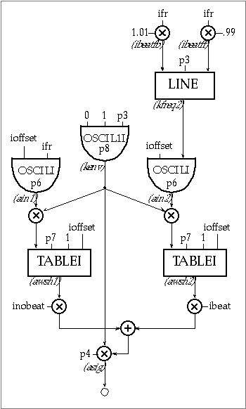
Figure 11.37 Block diagram of instr 1113, a dynamic waveshaping instrument.
| instr | 1113 | ; a dual waveshaping | ||
| ifr | = | cpspch(p5) | ; pitch to freq | |
| ioffset | = | .5 | ; offset | |
| ibeatfb | = | 1.01*ifr | ; begin value of beating freq | |
| ibeatff | = | 0.99*ifr | ; final value of beating freq | |
| inobeat | = | 0.8 | ; proportn non-beating oscil | |
| ibeat | = | 0.2 | ; proportn beating oscil | |
| kenv | oscil1i | 0, 1, p3, p8 | ; envelope (distortion index) | |
| kfreq2 | line | ibeatfb, p3, ibeatff | ; frequency change | |
| ain1 | oscili | ioffset, ifr, p6 | ; FIRST OSCILLATOR | |
| awsh1 | tablei | kenv*ain1, p7, 1, ioffset | ; waveshaping 1st oscil | |
| ain2 | oscili | ioffset, kfreq2, p6 | ; SECOND OSCILLATOR | |
| awsh2 | tablei | kenv*ain2, p7, 1, ioffset | ; waveshaping 2nd oscil | |
| asig | = | kenv*p4*(inobeat*awsh1+ibeat*awsh2) | ||
| out | asig | |||
| endin | ||||
Figure 11.38 Orchestra code for instr 1113, a dual waveshaping instrument.
In our example instr 1113 is composed of two waveshapers: the first one processes a sinewave of constant frequency f and the second processes a sinewave which varies its frequency throughout the duration of each note from 1.01f to 0.99f. The outputs of these waveshapers are mixed in a relative proportion of 0.8:0.2 (inobeat:ibeat), producing a variable beating pattern that further enhances the waveshaping process. The reader may notice that ioffset is 0.5 and not half of the table size minus one. This is because the table statements are used in normalized mode (the waveshaped signal varies between -0.5 and +0.5).
Summary
The following issues should be considered when implementing a waveshaping process:
1. Waveshaper function, which determines the amount of distortion as a function of amplitude. Chebyshev functions may be used with sinewaves in order to produce various combinations of harmonics. It is also possible to interpolate between two or more waveshaping functions by cross-fading the outputs.
2. Distortion index, which is essentially the envelope of the sound. It determines which region of the waveshaper is used at a given moment.
Frequency Modulation
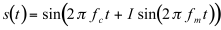
John Chowning (1973) initially proposed the application of frequency modulation (FM) to musical synthesis. He showed that the use of a modulator in order to modify the frequency of a carrier, may be controlled to produce varied dynamic spectra with relatively little computational overheads. In its simplest form, both the carrier and the modulator are sinewaves; however, unlike ring modulation, sinewave FM generates enough spectral complexity to allow the synthesis of reasonably rich and varied timbres. The mathematical expression for a signal of frequency fm, which modulates a carrier of frequency fc, is:
 (11.12)
Where I, called the modulation index, controls the degree of distortion applied to the carrier. Its function can be compared with that of the distortion index in waveshaping and will be discussed below.
Equation 11.12 may be manipulated by expressing the sine functions as a power series which, after a rather lengthy process, results in the following expression
 (11.13)
The equation above describes a spectrum with sidebands at frequencies fc± fm, fc±2fm, fc±3fm, etc. above and below the carrier fc, as shown in figure 11.39.
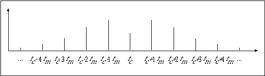
Figure 11.39 Spectrum of frequency modulation process.
The amplitude of each pair of components is determined by the coefficients J1, J2, J3, etc. which are functions of the index I. The actual mathematical dependency of Jn on I is given by a family of curves known as Bessel functions. (Mathematical expressions and a graphic representation of Bessel functions can be found in various calculus textbooks. Graphic plots are also shown in Chowning (1973)). In practice, the influence of I may be evaluated by means of a simple rule of thumb: the total number of audible sidebands is 2I (I sidebands above and I sidebands below the carrier). Therefore, the total number of components, including the carrier, is 2I+1. This is illustrated in 1114.orc and 1114.sco. The orchestra uses a foscili opcode to implement FM, where p5*p6 is the frequency of the carrier, p5*p7 is the frequency of the modulator, p8 is the index and p9 is the function table which generates the carrier and the modulator — a sinewave in this case.

Figure 11.40 Block diagram of instr 1114, a simple static FM instrument.
| instr | 1114 | ; simple static FM | ||
| kenv | linen | p4, .1, p3, .1 | ; env (attack = decay = .1 sec) | |
| asig | foscili | kenv, p5, p6, p7, p8, p9 | ; FM oscillator | |
| out | asig | ; output | ||
| endin | ||||
Figure 11.41 Orchestra code for instr 1114, a simple static FM instrument.
The score includes five examples of a 212 Hz modulator applied to a 100 Hz carrier, with respective index values of 0, 1, 2, 3 and 4. The first sound (I=0) contains the carrier alone, the second includes the first pair of sidebands, the third extends the spectrum to the next pair and so on. When 1114.sco is synthesized, it is possible to hear how the top frequency component becomes higher as more sidebands become audible. In short, the index determines how many components will be audible.
We saw above that ring modulation may generate negative frequencies. This also happens in Frequency Modulation (FM). In this case, formula 11.13 only contains sines (as opposed to cosines in ring modulation); therefore, from the trigonometric identity:
 (11.14)
we can infer that negative components reflect with a change of sign. This is equivalent to a phase shift of¹, or half a cycle.
The carrier to modulator ratio is also an important FM parameter. It has a similar effect on the output to that of the ring modulation c/m. If c/m is not a rational number, the spectrum will be inharmonic, but if the c/m can be represented as a ratio of integers
 (11.14)
then the fundamental will be f = fc/Nc = fm/Nm and the spectrum will be harmonic. Also, fc and fm will be respectively the Ncth and Nmth harmonics. However, if the fundamental f is below the auditory range, the sound will not be perceived as having definite pitch, as demonstrated in 1114a.orc and 1114a.sco, which use instr 1114 to produce the following three sounds:
| c=80Hz | c/m=1 | I=2 | Fundamental=80Hz | |
| c=80Hz | c/m=13/19 | I=2 | Fundamental=80/13=6.154Hz | Lacks clear pitch |
| c=80Hz | c/m=1.4142~ |
I=2 | Sound is inharmonic | |
Figure 11.42 Table of tutorial parameter values and description of their sound.
Furthermore, because the harmonic content depends on the difference between the carrier and multiples of the oscillator frequency, we can conclude that if Nm = 1, the spectrum will contain all the harmonics. If Nm is even, every second harmonic will be missing and the spectrum will contain f, 3f, 5f, etc. For example, if c/m = 1/2, then Nm = 2, f c =f and fm = 2f; therefore, the spectrum will only contain odd harmonics, which are the result of adding f to a multiple of 2f, as follows:
| f+2f = 3f | f-2f = -f |
| f+2x(2f) = 5f | f-2x(2f) = -3f |
| f+3x(2f) = 7f | f-3x(2f) = -5f |
| f+4x(2f) = 9f | f-4x(2f) = -7f |
| etc. | |
Figure 11.43 Table of odd partials resulting from a c/m ration of 1:2.
Similarly, if Nm=3, every third harmonic will be missing.
Dynamic FM spectra may be obtained by making c/m and I functions of time. In fact, a time-varying index alone provides enough versatility to produce a variety of sounds, as illustrated in 1115.orc and 1115.sco in which instr 1115 controls the envelope and the index using the variables kenv and kidx.
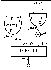
Figure 11.44 Block diagram of instr 1115, a dynamic FM instrument
| instr | 1115 | ; FM w/ amplitude and spectral envelopes | ||
| ifreq | = | cpspch(p5) | ; pitch to frequency | |
| kenv | oscil1 | 0, p4, p3, p11 | ; amplitude envelope | |
| kindx | oscil1 | 0, p8-p9, p3, p12 | ; time-varying index | |
| asig | foscili | kenv, ifreq, p6, p7, p9+kindx, p10 | ; FM oscillator | |
| out | asig | ; output | ||
| endin | ||||
Figure 11.45 Orchestra code for instr 1115, a dynamic FM instrument with amplitude and spectral envelopes.
The score file 1115.sco produces a passage that includes various types of sounds based on recipes for bells, woodwind, brass and membranophones, proposed by Chowning (1973). In these c/m is fixed for each type and only the index changes between a maximum and a minimum value (p8 and p9, respectively). The modulation-index, I, is driven by an oscillator with different generating functions given in the score, according to the desired type of sound. The overall amplitude envelope also plays an important role in modeling these sounds. For example, the sudden attack resulting from hitting the body of a bell and the subsequent slow decay into a pitched sound may be modeled using: an exponential amplitude envelope which lasts a few seconds; an inharmonic carrier-to-modulator ratio; and a modulation-index which initially favors high partials (kidx=6) and decays slowly to zero, gradually making the carrier more prominent (kidx=1.2). The amplitude and index envelopes are modeled with the following function tables:
| f 11 | 0 | 512 | 5 1 512 .0001 | ; bell amplitude |
| f 12 | 0 | 512 | 5 1 512 .2 | ; bell index |
The instrument statement below produces a 4-second bell using an inharmonic carrier to modulator ratio of 1/1.215 and a maximum index of 6.
| ; ins | st | dur | amp | ptch | c | m | max I | min I | osc fn | amp fn | ndx fn |
| i 1115 | 0 | 4 | 10000 | 8.01 | 1 | 1.215 | 6 | 0 | 1 | 11 | 12 |
Summary
There are two important parameters that determine the spectral characteristics of sounds produced by frequency modulation.
1. The carrier to modulator ratio determines the location of frequency components.
2. The index determines which components will be prominent.
Granular Synthesis
Granular synthesis theory was first developed by Gabor (1947), who argued that signals can be conceived as the combination of very short sonic grains. A particular grain may be indistinguishable from another grain; however, combinations of large numbers of these sonic units may yield different morphologies, depending on the internal constitution of the grains and on the particular way in which the combination is structured.
According to psychoacoustic theory, human perception becomes ineffective in recognizing pitch and amplitude when sonic events become too short: the threshold has been estimated to be in the region of 50 milliseconds (Whitfield 1978). Therefore, typical durations of grains usually fall between 10 to 60 milliseconds.
A grain usually consists of a waveform with an envelope, as shown in figure 11.47. In principle, the former could be any signal — ranging from pure sinewaves to recorded samples of complex sounds. The envelope can have various shapes — for example, it could be a Gaussian curve, a triangle, a trapezoid, half-a-sine, etc. When grains are combined, the shape of the waveform and envelope are influential factors which determine the timbre of the overall sonic result. As a rule of thumb, complex waveforms will lead to sounds with larger noise content. Also, envelopes with edges (such as triangles and trapezoids) will produce rougher signals. Furthermore, depending on the sampling rate, if the duration of a grain is very short, the attack and/or decay of a trapezoid may become vertical, causing clicks. On the other hand, smooth envelopes such as half-sine may be effective in preventing clicks at shorter durations.

Figure 11.46 Grains with triangular waveforms and Gaussian envelopes.
Because grains are short, it is necessary to manipulate these in large numbers to obtain any significant results; sometimes, the numbers may reach up to 1000 grains per second of sound. Therefore, it is useful to adopt high level organizational strategies that take care of the manipulation of the various parameters associated with grain characteristics and with their combination.
Throughout the history of electronic synthesis, there have been various approaches and, even now, new strategies are being developed. In the early sixties, Xenakis (1971) proposed organization of grains according to a synchronous process: time may be divided into frames which are then played in succession at a constant rate, similar to movie frames which produce continuous movement. Each frame consists of two axes — one of which measures frequency and the other amplitude — and contains a particular set of grains, each with its own amplitude-frequency values. Therefore, when the frames are ‘played,’ a particular succession of grains with varying frequency and density is obtained.
Another strategy, perhaps the most popular to date, consists of the creation of asynchronous "clouds," described in depth by Roads (1985, 1991). The main idea behind a cloud of grains is that the tendencies of the various parameters that influence the resulting musical sound may be controlled by means of a process that is partly random and partly deterministic. For example, a random device that produces values falling between a lower and upper limit determined by the composer may generate the frequency of the grain waveform. These limits may change in time, producing dynamic spectra.
The following list describes the most typical parameters:
• Grain duration: typically between 5 and 50 milliseconds. Values above this range may loose the ‘anonymity’ of grains and may be used effectively in order to create a transition between granular textures and gestural material. Grain duration may also produce ring modulation effects (Roads, 1991, pp. 157-161).
• Grain waveform type: which may vary from a pure sinewave to complex spectral types. In fact, the waveform of the grains may be made to change by interpolating gradually between two extreme cases. Another method of creating time-varying waveforms consists of using a frequency modulation unit with varying carrier to modulator ratio and FM index.
• Grain envelope: typical envelopes include bell-shaped Gaussians, raised sinusoidals and trapezoids (attack-sustain-decay).
• Cloud density: which is the number of grains per time unit. Since the cloud is asynchronous (grains do not occur at regular intervals): on the one hand, some grains may overlap and, on the other hand, lapses of silence may occur. It these lapses are very short, they will not be perceived as such but will rather as fluctuations in amplitude, affecting the timbre of the output.
• Cloud amplitude envelope: which controls the overall amplitude of the cloud. Furthermore, the relative amplitude of each grain may be made to fluctuate between minimum and maximum values.
• Cloud frequency band: the grain waveform frequency at any given moment may be constrained to a spectral band determined by two time-varying functions; one for the higher limit and one for the lower limit.
• Cloud spatial movement: which may be controlled according to the number of outputs available.
• Cloud width or grain spatial scatter: the localization of the cloud at any moment may vary from confinement to a point in space to wide spatial spread, according to the degree of scattering of the grains in relation to the path along which the cloud moves.
The files 1116.orc and 1116.sco produce a 20-second cloud created by using an instrument which implements the parameters described above. The overall envelope of the cloud is produced using an oscil1 statement with duration idur (p3) amplitude imaxamp (p4) and function iampfunc (p5)
| kenv | oscil1 | 0, imaxamp, idur, iampfunc | ; overall envelope |
The lower limit of the frequency band varies between a minimum ilfbmin and a maximum ilfbmax, given respectively by p11 and p12. The difference of these values, ilfbdiff, is fed to an oscil1 statement driven by function ilbffunc (p3). The output of the oscillator is then added to lbfmin in order to obtain the time-varying lower limit klbf.
| ilfbmin | = | p11 | ; minimum freq of limit |
| ilfbmax | = | p12 | ; maximum freq of limit |
| ilfbdiff | = | ilfbmax-ilfbmin | ; difference |
| ilbffunc | = | p13 | ; lower limit function |
| klfb | oscil1 | 0, ilfbdiff, idur, ilbffunc | ; lower limit fluctuatn |
| klfb | = | ilfbmin+klfb | ; lower limit |
A similar procedure is applied in order to produce the upper limit of the frequency band (kufb), the carrier-to-modulator ratio (kcmr), the index (kidx) and the width of the cloud (kgscat).
Spatialization of the cloud is implemented using the same algorithm employed in the dynamic additive synthesis instrument described previously in this chapter. The only difference consists of the addition of grain scatter to the overall panning.
| kpan | = | kpan+kgscat | ; add grain scatter |
Applying a periodic envelope to an otherwise continuous sound produces the grains. The rate at which the grains are produced is the same as the frequency of the envelope generator; therefore, if the duration of the grain is kgdur, the rate at which the envelope for that grain is generated is kgrate = 1 /kgdur. The code used to control the grain duration is listed below:
| imingd | = | p6/1000.0 | ; minimum grain duration |
| imaxgd | = | p7/1000.0 | ; maximum grain duration |
| igddiff | = | imaxgd-imingd | ; difference |
| igdfunc | = | p8 | ; grain duration func table |
| kgdur | oscil1 | 0, igddiff, idur, igdfunc | ; grain duration fluctuation |
| kgdur | = | imingd+kgdur | ; grain duration |
| kgrate | = | 1.0/kgdur | ; grain rate |
Since p6 and p7 give the minimum and maximum grain duration in milliseconds, it is necessary to divide these by 1000 in order to obtain imingd and imaxgd in seconds. The maximum fluctuation in grain duration is igddiff, which is used as amplitude for an oscillator driven by the grain duration function igdfunc (p8). Therefore, kgdur is the result of adding the output of the oscillator to the minimum duration imingd. Finally, kgrate is calculated.
The grain envelope uses kgrate as its frequency and igefunc (p10) as the generating function table.
| igefunc | = | p10 | ; grain envelope func table |
| kgenvf | = | kgrate | ; grain envelope frequency |
| kgenv | oscili | 1.0, kgenvf, igefunc | ; envelope |
Also, kgrate is used to generate the relative amplitude and waveform frequency of the grain. Using a randh statement, which produces values between specified maxima and a minima, does this. The relative amplitude consists of a scaling factor which may assume values between hmaxfc (=0.5) and 1.
| ihmaxfc | = | 0.25 | ; half of maximum amplitude dev |
| kgafact | randh | ihmaxfc, kgfreq, iseed/3 | ; -ihmaxfc<rand number<+ihmaxfc |
| kgafact | = | 1.00-(ihmaxfc+kgafact) | ; 2*ihmaxfc<scaling factor<1.00 |
The waveform frequency assumes a random value between the low and high limits of the cloud’s frequency band (klfb and kufb).
| kgband | = | kufb-klfb | ; current frequency band |
| kgfreq | randh | kgband/2, kgrate, iseed | ; generate frequency |
| kgfreq | = | klfb+kgfreq+kgband/2 | ; frequency |
A grain is generated using a foscili opcode, which uses the cloud’s instantaneous carrier-to-modulator ratio and index (kcmr and kidx).
| igfunc | = | p9 | ; grn. wave fn |
| agrain | foscili | kgenv, kgfreq, 1, kcmr, kidx, igfunc | ; FM generator |
In order to avoid mechanical repetition and achieve grain overlap, a random variable delay is applied to each generated grain. The maximum possible delay value is equal to the grain duration (kgdur). The actual delay is produced using a randi generator.
| kgdel | randi | kgdur/2, kgrate, iseed/2 | ; random sample delay |
| kgdel | = | kgdel+kgdur/2 | ; make it positive |
| adump | delayr | imaxgd | ; delay line |
| adelgr | deltapi | kgdel | |
| delayw | kgafact*agrain | ||
After the grain is delayed, an additional delay line applies Doppler shift to the moving grain according to its spatial position kpan. This assumes a speaker distance of 10 meters.
| ihspeakd | = | 5.0 | ; halfspkrsdistnce(m) | |
| isndsp | = | 331.45 | ; soundspeedinair(m/sec) | |
| impandel | = | (imaxpan+imaxscat)*ihspeakd/isndsp | ; max pan delay | |
| kpdel | = | kpan*ihspeakd/isndsp | ; find pan delay | |
| adump | delayr | impandel | ; set max dopplerdelay | |
| agdop | deltapi | abs(kpdel) | ; tapdelay via panval | |
| delayw | adelgr | ; delay signal | ||
To create the left and right channels the output of the Doppler processor is then multiplied by kpleft and kpright.
| asig | = | kenv*agdop |
| outs | kpleft*asig, kpright*asig |
The cloud generated by 1116.sco has an amplitude envelope that is half of a sinewave. The grain duration varies between 10 and 30 milliseconds: initially, grains assume the longer duration, which becomes shorter towards the middle section and then increases up to about 24 msec., shortening slightly towards the end to 21 msec. The frequency band is initially very narrow, around 2500 Hz, widening and narrowing as the sound progresses, with a lower boundary which varies between a minimum of 1000 Hz and a maximum of 2500 Hz and an upper boundary which varies between 2500 and 4670 Hz. The carrier-to-modulator ratio assumes an initial value of 1 and progresses for 1.25 seconds towards 4, its maximum value; it then hovers between a minimum of 1.48 and a maximum of 2.911. The FM index changes between 1 and 8, reaching the maximum (producing higher frequency components) after 12.5 seconds. Also f 9 controls the spatial movement in the stereo field, including Doppler shift and f 10 controls the scattering of grains by means of a sinusoidal with its second harmonic. This means that maximum scatter happens at about 2.5 and 17.5 seconds — which correspond respectively to 1/8th and 7/8ths of a cycle — and minimum scatter happens in the vicinity of 10 seconds (half a cycle).
Summary
The following parameters are typically used to control the characteristics of a cloud of grains:
1. Grain duration.
2. Grain waveform type (which may be varied using different techniques such as FM synthesis).
3. Grain envelope.
4. Cloud density.
5. Cloud amplitude.
6. Envelope.
7. Cloud frequency band.
8. Cloud spatial movement.
9. Cloud width (grain spatial scattering).
Conclusion
This chapter surveyed ‘classic’ synthesis techniques that derive from the capabilities of devices available in the early stages of electroacoustic music development. These may be classified into frequency-domain and time-domain techniques. Frequency-domain techniques can be linear — including additive and subtractive synthesis, or non-linear, including ring-modulation, waveshaping and frequency modulation. The most popular time-domain ‘classic’ technique is granular synthesis.
Although the above techniques are called ‘classic,’ they are by no means a thing of the past. In fact some of these are only beginning to fulfill their true potential since the advent of computer systems with fast processing speeds, which have given a new lease of life and extended the possibilities they offer, particularly in the generation of dynamic complex spectra. Subtractive and additive principles have developed into sophisticated mechanisms such as linear predictive code (LPC) and phase vocoding. The combination of subtractive and granular synthesis has led to the development of formant wave function synthesis (FOF) and wavelet analysis and synthesis. Furthermore, given that different techniques are conductive to the synthesis of different classes of sounds, combinations of ‘classic’ procedures are effectively used to achieve sonorities that would be extremely difficult — if not impossible — to realize by means of a single technique.
Therefore, truly understanding ‘classic’ techniques is essential in order to comprehend the possibilities offered by new technology and use this to achieve new and interesting timbral resources — particularly given the many interesting and complex hybrid combinations.
Finally, the reader should realize that composition is not only about sounds on their own; new sonorities are also the result of context. Thus, far from being concerned only with the internal properties of sonic structures, electroacoustic composition is more than ever dependent on the way sounds are combined with each other, on how they interact and on the way they can be used to shape time.
References
Backus, J. 1977. The Acoustical Foundations of Music. New York: W. W. Norton & Company, Inc.
Chowning, J. 1985. "The synthesis of complex audio spectra by means of frequency modulation." Journal of the Audio Engineering Society 21:526-534. Reprinted in C. Roads and J. Strawn, eds. Foundations of Computer Music. Cambridge, MA: M.I.T. Press. pp. 6-29.
Dodge, C. and T. Jerse. 1985. Computer Music, Synthesis Composition and Performance. New York: Schirmer Books, Macmillan Inc.
Fischman, R. 1991. Musical applications of digital synthesis and processing techniques. realization using csound and the phase vocoder. Keele: unpublished.
Gabor, D. 1947. "Acoustical quanta and the theory of hearing," Nature. 159 (4044): 591-594.
Roads, C. 1985. "Granular synthesis of sound." in C. Roads and J. Strawn, eds. 1985. Foundations of Computer Music. Cambridge, MA: M.I.T. Press. pp.145-159.
Roads, C. 1991 "Asynchronous granular synthesis." in G. De Poli, A. Piccialli and C. Roads, eds. Representation of Musical Signals. Cambridge, MA: M.I.T. Press. pp. 143-186.
Vercoe, B. 1993. Csound. Software and manual. Cambridge, MA: M.I.T. Press.
Whitfield, J. 1978. "The neural code." In E. Carterette and M. Friedman, eds. 1978. Handbook of Perception, Vol. IV, Hearing. Orlando: Academic.
Williams, C. S. 1986. Designing Digital Filters. New York: Prentice Hall, Inc.
Wishart, T. 1985. On Sonic Art. York: Imagineering Press.
Xenakis, I. 1971. Formalized Music. Bloomington: Indiana University Press.